Survival Regression

IN THIS CHAPTER

Knowing when to use survival regression

Grasping the concepts behind survival regression

Running and interpreting the outcome of survival regression

Peeking at prognosis curves

Estimating sample size for survival regression

Survival regression is one of the most commonly used techniques in biostatistics. It overcomes the limitations of the log-rank test (see Chapter 22) and allows you to analyze how survival time is influenced by one or more predictors (the X variables), which can be categorical or numerical. In this chapter, we introduce survival regression. We specify when to use it, describe its basic concepts, and show you how to run survival regressions in statistical software and interpret the output. We also explain how to build prognosis curves and estimate the sample size you need to support a survival regression.

Note: Because time-to-event data so often describe actual survival, when the event we are talking about is death, we use the terms death and survival time. But everything we say about death applies to the first occurrence of any event, like pre-diabetes patients restoring their blood sugar to normal levels, or cancer survivors suffering a recurrence of cancer.

Knowing When to Use Survival Regression

In Chapter 21, we examine the special problems that come up when the researcher can’t continue to collect data during follow-up on a participant long enough to observe whether or not they ever experience the event being studied. To recap, in this situation, you should censor the data. This means you should acknowledge the participant was only observed for a limited amount of time, and then was lost to follow-up. In that chapter, we also explain how to summarize survival data using life tables and the Kaplan-Meier method, and how to graph time-to-event data as survival curves. In Chapter 22, we describe the log-rank test, which you can use to compare survival among a small number of groups — for example, participants taking drug versus placebo, or participants initially diagnosed at four different stages of the same cancer.

But the log-rank test has limitations:

• The log-rank test doesn’t handle numerical predictors well. Because this test compares survival among a small number of categories, it does not work well for a numerical variable like age. To compare survival among different age groups with the log-rank test, you would first have to categorize the participants into age ranges. The age ranges you choose for your groups should be based on your research question. Because doing this loses the granularity of the data, this test may be less efficient at detecting gradual trends across the whole age range.
• The log-rank test doesn’t let you analyze the simultaneous effect of different predictors. If you try to create subgroups of participants for each distinct combination of categories for more than one predictor (such as three treatment groups and three diagnostic groups), you will quickly see that you have too many groups and not enough participants in each group to support the test. In this example — with three different treatment groups and three diagnostic groups — you would have 3 × 3 groups, which is nine, and is already too many for a log-rank test to be useful. Even if you have 100 participants in your study, dividing them into nine categories greatly reduces the number of participants in each category, making the subgroup estimate unstable.

Use survival regression when the outcome (the Y variable) is a time-to-event variable, like survival time. Survival regression lets you do all of the following, either in separate models or simultaneously:

• Determine whether there is a statistically significant association between survival and one or more other predictor variables
• Quantify the extent to which a predictor variable influences survival, including testing whether survival is statistically significantly different between groups
• Adjust for the effects of confounding variables that also influence survival
• Generate a predicted survival curve called a prognosis curve that is customized for any particular set of values of the predictor variables

Grasping the Concepts behind Survival Regression

Note: Our explanation of survival regression has a little math in it, but nothing beyond high school algebra. In laying out these concepts, we focus on multiple survival regression, which is survival regression with more than one predictor. But everything we say is also true when you have only one predictor variable.

Most kinds of regression require you to write a formula to fit to your data. The formula is easiest to understand and work with when the predictors appear in the function as a linear combination in which each predictor variable is multiplied by a coefficient, and these terms are all added together (perhaps with another coefficient, called an intercept, thrown in). Here is an example of a typical regression formula: . Linear combinations (such as c₂x₂ from the example formula) can also have terms with higher powers — like squares or cubes — attached to the predictor variables. Linear combinations can also have interaction terms, which are products of two or more predictors, or the same predictor with itself.

Survival regression takes the linear combination and uses it to predict survival. But survival data presents some special challenges:

• Censoring: Censoring happens when the event doesn’t occur during the observation time of the study (which, in human studies, means during follow-up). Before considering using survival regression on your data, you need to evaluate the impact censoring may have on the results. You can do this using life tables, the Kaplan-Meier method, and the log-rank test, as described in Chapters 21 and 22.
• Survival curve shapes: Some business disciplines develop models for estimating time to failure of mechanical or electronic devices. They estimate the times to certain kinds of events, like a computer’s motherboard wearing out or the transmission of a car going kaput, and find that they follow remarkably predictable shapes or distributions (the most common being the Weibull distribution, covered in Chapter 24). Because of this, these disciplines often use a parametric form of survival regression, which assumes that you can represent the survival curves by algebraic formulas. Unfortunately for biostatisticians, biological data tends to produce nonparametric survival curves whose distributions can’t be represented by these parametric distributions.

As described earlier, nonparametric survival analyses using life tables, Kaplan-Meier plots, and log-rank tests are limiting. But as biostatisticians, we could not rely on using parametric distributions in our models; we wanted to use a hybrid, semi-parametric kind of survival regression. We wanted one that was partly nonparametric, meaning it didn’t assume any mathematical formula for the shape of the overall survival curve, and partly parametric, meaning we could use some parameter (or predicted survival distribution shape) to guide our formulas the way other industries used the Weibull distribution. In 1972, a statistician named David Cox developed a workable method for doing this. The procedure is now called Cox proportional hazards regression, which we call PH regression for the rest of this chapter for brevity. In the following sections, we outline the steps of performing a PH regression.

Since 1972, many issues have been identified when using survival regression for biological data, especially with respect to its appropriateness for the type of data. One way to examine this is by running a logistic regression model (see Chapter 18) with the same predictors and outcome as your survival regression model without including the time variable, and seeing if the interpretation changes.

The steps to perform a PH regression

You can understand PH regression in terms of several conceptual steps, although when using statistical software like is described in Chapter 4, it may appear that these steps take place simultaneously. That is because the output created is designed for you — the biostatistician — to walk through the following steps in your mind and make decisions. You must use the output to:

1. Determine the shape of the overall survival curve produced from the Kaplan-Meier method.
2. Estimate how your hypothesized predictor variables may impact the bends in this curve — in other words, in what ways your predictors may affect survival.
3. Create a PH regression model that fits your data the best it can, and interpret the values of the regression coefficients so you can calculate predicted survival times.

Determining the baseline in time-to-event analyses

Your software may define the baseline survival function in one of two ways:

• The survival curve of an average participant: This curve is calculated as if the value of each predictor is equal to the group average value for that variable. The average-participant baseline is like the overall survival curve you get from a Kaplan-Meier calculation by using all the available participants.
• The survival curve of a hypothetical zero participant: This curve is calculated assuming the value of each predictor is equal to 0. Some mathematicians prefer to use the zero-participant baseline because can make formulas simpler, but biostatisticians don’t like it because it corresponds to a hypothetical participant who can’t possibly exist in the real world. No actual person has an age equal to 0 years, or weighs 0 kilograms, and so on. The survival curve for this impossible person doesn’t look like a regular survival curve, so as biostatisticians, we can’t really use the zero-participant baseline survival function.

Luckily, the way your software defines its baseline function doesn’t affect any of the calculated measures on your output, so you don’t have to worry about it. But you should be aware of these definitions if you plan to generate prognosis curves, because the formulas to generate these are slightly different depending upon the way the computer calculates the baseline survival function.

Bending the baseline

Now for the tricky part. How do you bend or flex this baseline curve to express how survival may increase or decrease for different predictor values? Survival curves always start at 1.0 at time 0, meaning 100 percent of the sample do not have the event at time 0. The bending process must preserve that time starts at 0, and maximum survival is 1.0. If you raise 0 or 1 to any power, you will find that they stay the same — 0 stays 0, and 1 stays 1. But, exponentiating any number between 0 and 1 smoothly raises or lowers all the values between 0 and 1.

We will demonstrate what we mean by imagining our baseline function was a straight line (even though no actual biological survival curve would ever be exactly a straight line). Look at Figure 23-1a, which is a graph of the equation .

To understand the flex, look at what happens when you raise this straight line to various powers, which we refer to as h and illustrate in Figure 23-1b:

• Squaring: If you set h = 2, the y value for every point on the line always comes out smaller, because they are always less than 1. For example, is 0.64.
• Taking the square root: If we set h = 0.05, the y value of every point on the line becomes larger. For example, the square root of 0.25 is 0.5.

Notice in Figure 23-1b, both and remain 1, and and both remain 0, so those two ends of the line don’t change.

Does the same trick work for a survival curve that doesn’t follow any particular algebraic formula? Yes, it does! Look at Figure 23-2.

Here are some important points about Figure 23-2:

• Figure 23-2a shows a typical survival curve. It’s not defined by any algebraic formula. It just graphs the table of values obtained by a life-table or Kaplan-Meier calculation.
• Figure 23-2b shows how the baseline survival curve is flexed by raising every baseline survival value to a power. You get the lower curve by setting h = 2 and squaring every baseline survival value. You get the upper curve by setting h = 0.05 and taking the square root of every baseline survival value. Notice that the two flexed curves keep all the distinctive zigs and zags of the baseline curve, in that every step occurs at the same time value as it occurs in the baseline curve.
  • The lower curve represents a group of participants who had a worse survival outcome than those making up the baseline group. This means that at any instant in time, they were somewhat more likely to die than a baseline participant at that same moment. Another way of saying this is that the participants in the lower curve have a higher hazard rate than the baseline participants.
  • The upper curve represents participants who had better survival than a baseline person at any given moment — meaning they had a lower hazard rate.

Obviously, there is a mathematical relationship between the chance of dying at any instant in time, which is called hazard, and the chance of surviving up to some point in time, which we call survival. It turns out that raising the survival curve to the h power is exactly equivalent to multiplying the hazard curve by the natural logarithm of h. Because every point in the hazard curve is being multiplied by the same amount — by Log(h) — raising a survival curve to a power is referred to as a proportional hazards transformation.

But what should the value of h be? The h value varies from one individual to another. Keep in mind that the baseline curve describes the survival of a perfectly average participant, but no individual is completely average. You can think of every participant in the data as having her very own personalized survival curve, based on her very own h value, that provides the best estimate of that participant’s chance of survival over time.

Seeing how predictor variables influence h

The final piece of the PH regression puzzle is to figure out how the predictor variables influence h, which influences survival. As you likely know, all regression procedures estimate the values of the coefficients that make the predicted values agree as much as possible with the observed values. For PH regression, the software estimates the coefficients of the predictor variables that make the predicted survival curves agree as much as possible with the observed survival times of each participant.

How does PH regression determine these regression coefficients? The short answer is, “You’ll be sorry you asked!” The longer answer is that, like all other kinds of regression, PH regression is based on maximum likelihood estimation. The software uses the data to build a long, complicated expression for the probability of one particular individual in the data dying at any point in time. This expression involves that individual’s predictor values and the regression coefficients. Next, the software constructs a longer expression that includes the likelihood of getting exactly the observed survival times for all the participants in the data set. And if this isn’t already complicated enough, the expression has to deal with the issue of censored data. At this point, the software seeks to find the values of the regression coefficients that maximize this very long likelihood expression (similar to the way maximum likelihood is described with logistic regression in Chapter 18).

Executing a Survival Regression

As with all statistical methods dealing with time-to-event data, your dependent variable is actually a pair of variables:

• Event status: The event status variable is coded this way:
  • Equal to 1 if the event was known to occur during the observation period (uncensored)
  • Equal to 0 if the event didn’t occur during the observation period (censored)
• Time-to-event: In participants who experienced the event during the observation period, this is the time from the start of observation to the occurrence of the event. In participants who did not experience the event during the observation period, this is the time from the start of observation to the last time the participant was observed. We describe time-to-event data in more detail in Chapter 21.

And as with all regression methods, you designate one or more variables as the predictors. The rules for representing the predictor variables are the same as described in Chapter 18:

• For continuous numerical variables, choose units of a convenient magnitude.
• For categorical predictors, carefully consider how you recode the data, especially in terms of selecting a reference group. Consider a five-level age group variable. Would you want to model it as an ordinal categorical variable, assuming a linear relationship with the outcome? Or would you prefer using indicator variables, allowing each level to have its own slope relative to the reference level? Flip to Chapter 8 for more on recoding categorical variables.

You may not be sure which variables in your data to include as predictors in the regression. We provide advice on model-building in Chapter 17.

After you assemble and properly code the data, you execute the regression in statistical software using a similar approach as you use when doing ordinary least-squares or logistic regression. You need to specify the variables in the regression model:

1. Specify the two outcome variables.
   • The event status variable
   • The time-to-event variable

2. Specify the predictor variables.

   Make sure you are careful when you include categorical predictors, especially indicator variables. All the predictors you introduce should make sense together in the model.

Most software also lets you specify calculations you want to see on the output. You should always request at least the following:

• Coefficients table, including HRs and their confidence intervals
• Tests of whether the hazard proportionality assumption is valid

You may also want to request the following output:

• Summary descriptive statistics about the data. These can include number of censored and uncensored observations, median survival time, and mean and standard deviation for each predictor variable in the model
• One or more measures of goodness-of-fit for the model
• Baseline survival function, which outputs as a table of values and a survival curve
• Baseline hazard function values, which output as a table and graph

After you specify all the input to the program, execute the code, retrieve the output, and interpret the results.

Interpreting the Output of a Survival Regression

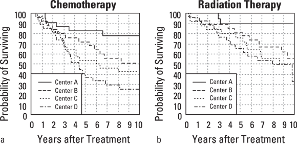
Suppose that you have conducted a long-term survival study of 200 Stage 4 cancer patients who were enrolled from four clinical centers (A, B, C, and D) and were randomized to receive either chemotherapy or radiation therapy. Participants were followed for up to ten years, after which the survival data were summarized by treatment (see Figures 23-3a and 23-3b for the two treatments) and by clinical center.

It would appear, from Figure 23-3, that radiation (compared to chemotherapy) and clinical centers A and B (compared to C and D) are associated with better survival. But are these apparent effects statistically significant? PH regression can answer these and other questions.

To run a PH regression on the data from this example, you must indicate the following to the software in your code:

• The time-to-event variable. We named this variable Time, and it was coded in years. For participants who died during the observation period, it was coded as the number of years from observation beginning until death. For participants who did not die during the observation period, it contains number of years they were observed.
• The event status variable. We named this variable Status, and coded it as 1 if the participant was known to have died during the observation period, and 0 if they did not die.
• The treatment group variable. In this case, we created the variable Radiation, and coded it as 1 if the participant was in the radiation group, and 0 if they were in the chemotherapy group. That way, the coefficient produced in the output will indicate the increase or decrease in proportional hazard associated with being in the radiation group compared to the chemotherapy group.
• The clinical center variable. In this case, we choose to create an indicator variable called CenterCD, which is 1 if the participant is from Center C or Center D, and is 0 if they are from A or B. Alternatively, you could choose to create one indicator variable for each center, as described in Chapter 18.

If you use a numerical variable such as age as a predictor and enter it into the model, the resulting coefficient will apply to increasing this variable by one unit (such as for one year of age).

Using the R statistical software, the PH regression can be invoked with a single command:

coxph(formula = Surv(Time, Status) ~ CenterCD + Radiation)

Figure 23-4 shows R’s output, using the data that we graph in Figure 23-3. The output from other statistical programs won’t look exactly like Figure 23-4, but you should be able to find the main components described in the following sections.

Testing the validity of the assumptions

When you’re analyzing data using PH regression, you’re assuming that your data are consistent with the idea of flexing a baseline survival curve by raising all the points in the entire curve to the same power (shown as h in Figures 23-1b and 23-2b). You’re not allowed to twist the curve so that it goes higher than the baseline curve () for small time values and lower than baseline () for large time values. That would be a non-PH flexing of the curve.

One quick check to see whether a predictor is affecting your data in a non-PH way is to take the following steps:

1. Split your data into two groups, based on the predictor.

2. Plot the Kaplan-Meier survival curve for each group (see Chapter 22).

   If the two survival curves for a particular predictor display the slanted figure-eight pattern shown in Figure 23-5, either don’t use PH regression on those data, or don’t use that predictor in your PH regression model. That’s because it violates the assumption of proportional hazards underlying PH regression.

Your statistical software may offer several options to test the hazard-proportionality assumption. Check your software’s documentation to see what it offers and how to interpret the output. It may offer the following:

• Graphs of the hazard functions versus time, which let you see the extent to which the hazards are proportional.
• A statistical test for significant hazard non-proportionality. R provides a function called cox.zph for this purpose, and other packages may offer a comparable option.

How Long Have I Got, Doc? Constructing Prognosis Curves

A primary reason to use regression analysis is to predict outcomes from any particular set of predictor values. For survival analysis, you can use the regression coefficients from a PH regression along with the baseline survival curve to construct an expected survival (prognosis) curve for any set of predictor values.

Suppose that you’re survival time (from diagnosis to death) for a group of cancer patients in which the predictors are age, tumor stage, and tumor grade at the time of diagnosis. You’d run a PH regression on your data and have the program generate the baseline survival curve as a table of times and survival probabilities. After that, whenever a patient is newly diagnosed with cancer, you can take that person’s age, stage, and grade, and generate an expected survival curve tailored for that particular patient. (The patient may not want to see it, but at least it could be done.)

You’ll probably have to do these calculations outside of the software that you use for the survival regression, but the calculations aren’t difficult and can be done in a Microsoft Excel spreadsheet. The example in the following sections uses the small set of sample data that’s preloaded into the online calculator for PH regression at https://statpages.info/prophaz.html. This particular example has only one predictor, but the basic idea extends to multiple predictors.

Obtaining the necessary output

Figure 23-6 shows the output from the built-in example (omitting the Iteration History and Overall Model Fit sections). Pretend that this model represents survival, in years, as a function of age for patients just diagnosed with some particular disease. In the output, the age variable is called Variable 1.

Looking at Figure 23-6, first consider the table in the Baseline Survivor Function section, which has two columns: time in years, and predicted survival expressed as a fraction. It also has four rows — one for each time point in which one or more deaths was actually observed. The baseline survival curve for the example data starts at 1.0 (100 percent survival) at time 0, as survival curves always do, but this row isn’t shown in the output. The survival curve remains flat at 100 percent until year two, when it suddenly drops down to 99.79 percent, where it stays until year seven, when it drops down to 98.20 percent, and so on.

In the Descriptive Stats section near the start of the output in Figure 23-6, the average age of the 11 patients in the example data set is 51.1818 years, so the baseline survival curve shows the predicted survival for a patient who is exactly 51.1818 years old. But suppose that you want to generate a survival curve that’s customized for a patient who is a different age — like 55 years old. According to the PH model, you need to raise the entire baseline curve to some power h. This means you have to exponentiate the four tabulated points by h.

In general, h depends on two factors:

• The value of the predictor variable for that patient. In this example, the value of age is 55.
• The values of the corresponding regression coefficients. In this example, in Figure 23-6, you can see 0.3770 labeled as Coeff. in the regression table.

Estimating the Required Sample Size for a Survival Regression

Note: Elsewhere in this chapter, we use the word power in its algebraic sense, such as in is x to the power of 2. But in this section, we use power in its statistical sense to mean the probability of getting a statistically significant result when performing a statistical test.

Except for straight-line regression discussed in Chapter 16, sample-size calculations for regression analysis tend not to be straightforward. If you find software that will calculate sample-size estimates for survival regression, it often asks for inputs you don’t have.

Very often, sample-size estimates for studies that use regression methods are based on simpler analytical methods. We recommend that when you’re planning a study that will be analyzed using PH regression, you base your sample-size estimate on the simpler log-rank test, described in Chapter 22. The free PS program handles these calculations very well.

You still have to specify the following:

• Desired α level: We recommend 0.05
• Desired power: We usually use 80 percent
• Effect size of importance: This is typically expressed as a HR or as the difference in median survival time between groups

You also need estimates of the following:

• Anticipated enrollment rate: How many participants you hope to enroll per time period
• Planned duration of follow-up: How long you plan to continue following all the participants after the last participant has been enrolled before ending the study and analyzing your data

If you are uncomfortable with estimating sample size for a large study that will be evaluated with a regression model, consult a statistician with experience in developing sample-size estimates for similarly-designed studies. They will be able to guide you in the tips and tricks they use to arrive at an adequate sample-size calculation given your research question and context.