Chapter 18
A Yes-or-No Proposition: Logistic Regression
IN THIS CHAPTER
 Figuring out when to use logistic regression
Getting a grip on the basics of logistic regression
Running a logistic regression model and making sense of the output
Watching for common issues with logistic regression
Estimating the sample size you need for logistic regression
You can use logistic regression to analyze the relationship between one or more predictor variables (the X variables) and a categorical outcome variable (the Y variable). Typical categorical outcomes include the following two-level variables (which are also called binary or dichotomous):
- Lived or died by a certain date
- Did or didn’t get diagnosed with Type II diabetes
- Responded or didn’t respond to a treatment
- Did or did not choose a particular health insurance plan
In this chapter, we explain logistic regression. We describe the circumstances under which to use it, the important related concepts, how to execute it with software, and how to interpret the output. We also point out the pitfalls with logistic regression and show you how to determine the sample sizes you need to execute such a model.
Using Logistic Regression
Following are typical uses of logistic regression analysis:
- To test whether one or more predictors and an outcome are statistically significantly associated. For example, to test whether age and/or obesity status are associated with increased likelihood to be diagnosed with Type II diabetes.
- To overcome the limitations of the 2x2 cross-tab method (described in Chapter 12), which can analyze only one predictor at a time (and the predictor has to be binary). With logistic regression, you can analyze multiple predictor variables at a time. Each predictor can be a numeric variable or a categorical variable having two or more levels.
- To quantify the extent or magnitude of an association between a particular predictor and an outcome that have been established to have an association. In other words, you are seeking to quantify the amount by which a specific predictor influences the chance of getting the outcome. As an example, you could quantify the amount obesity plays a role in the likelihood of a person being diagnosed with Type II diabetes.
- To develop a formula to predict the probability of getting an outcome based on the values of the predictor variables. For example, you may want to predict the probability that a person will be diagnosed with Type II diabetes based on the person’s age, gender, obesity status, exercise status, and medical history.
- To make yes or no predictions about the outcome that take into account the consequences of false-positive and false-negative predictions. For example, you can generate a tentative cancer diagnosis from a set of observations and lab results using a formula that balances the different consequences of a false-positive versus a false-negative diagnosis.
- To see how one predictor influences the outcome after adjusting for the influence of other variables. One example is to see how the number of minutes of exercise per day influences the chance of having a heart attack after controlling for the for the effects of age, gender, lipid levels, and other patient characteristics that could influence the outcome.
- To determine the value of a predictor that produces a certain probability of getting the outcome. For example, you could determine the dose of a drug that produces a favorable clinical response in 80 percent of the patients treated with it, which is called the
 , or 80 percent effective dose.
Understanding the Basics of Logistic Regression
In this section, we explain the concepts underlying logistic regression using an example from a fictitious animal study involving data on mortality due to radiation exposure. This example illustrates why straight-line regression wouldn’t work and why you have to use logistic regression instead.
Gathering and graphing your data
As in the other chapters in Part 5, we present a real-world problem here. This example examines the lethality of exposure to gamma-ray radiation when given in acute, large doses. It is already known that gamma-ray radiation is deadly in large-enough doses, so this animal study is focused only at the short-term lethality of acute large doses. Table 18-1 presents data on 30 animals in two columns.
TABLE 18-1 Radiation Dose and Survival Data for 30 Animals, Sorted Ascending by Dose Level
Dose in REMs |
Outcome |
Dose in REMS |
Outcome |
|---|---|---|---|
0 |
0 |
433 |
0 |
10 |
0 |
457 |
1 |
31 |
0 |
559 |
1 |
82 |
0 |
560 |
1 |
92 |
0 |
604 |
1 |
107 |
0 |
632 |
0 |
142 |
0 |
686 |
1 |
173 |
0 |
691 |
1 |
175 |
0 |
702 |
1 |
232 |
0 |
705 |
1 |
266 |
0 |
774 |
1 |
299 |
0 |
853 |
1 |
303 |
1 |
879 |
1 |
326 |
0 |
915 |
1 |
404 |
1 |
977 |
1 |


In Table 18-1, dose is the radiation exposure expressed in units called Roentgen Equivalent Man (REM). Because Table 18-1 is sorted ascending by dose, by looking at the Dose and Outcome columns, you can get a rough sense of how survival depends on dose. At low levels of radiation, almost all animals live, and at high doses, almost all animals die.
How can you analyze these data with logistic regression? First, make a scatter plot (see Chapter 16) with the predictor — the dose — on the X axis, and the outcome of death on the Y axis, as shown in Figure 18-1a.

© John Wiley & Sons, Inc.
FIGURE 18-1: Dose versus mortality from Table 18-1: each individual’s data (a) and grouped (b).
In Figure 18-1a, because the outcome variable is binary, the points are restricted to two horizontal lines, making the graph difficult to interpret. You can get a better picture of the dose-lethality relationship by grouping the doses into intervals. In Figure 18-1b, we grouped the intervals into 200 REM classes (see Chapter 9), and plotted the fraction of individuals in each interval who died. Clearly, Figure 18-1b shows the chance of dying increases with increasing dose.
Fitting a function with an S shape to your data
 Don’t try to fit a straight line if you have a binary outcome variable because the relationship is almost certainly not a straight line. For one thing, the fraction of individuals who are positive for the outcome can never be smaller than 0 nor larger than 1. In contrast, a straight line, a parabola, or any polynomial distribution would very happily violate those limits at extreme doses, which is obviously illogical.
If you have a binary outcome, you need to fit a function that has an S shape. The formula calculating Y must be an expression involving X that — by design — can never produce a Y value outside of the range from 0 to 1, no matter how large or small X may become.
 Of the many mathematical expressions that produce S-shaped graphs, the logistic function is ideally suited to this kind of data. In its simplest form, the logistic function is written like this:
 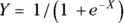 , where e is the mathematical constant 2.718, known as a natural logarithm (see Chapter 2). We will use e to represent this number for the rest of the chapter. Figure 18-2a shows the shape of the logistic function.
The logistic function shown in Figure 18-2 can be made more versatile for representing observed data by being generalized. The logistic function is generalized by adding two adjustable parameters named a and b like this: 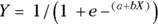 .
.

© John Wiley & Sons, Inc.
FIGURE 18-2: The first graph (a) shows the shape of the logistic function. The second graph (b) shows that when b is 0, the logistic function becomes a horizontal straight line.
Notice that the  part looks just like the formula for a straight line (see Chapter 16). It’s the rest of the logistic function that bends the straight line into its characteristic S shape. The middle of the S (where
  ) always occurs when
  . The steepness of the curve in the middle region is determined by b, as follows:
- If b is positive, the logistic function is an upward-sloping S-shaped curve, like the one shown in Figure 18-2a.
- If b is 0, the logistic function is a horizontal straight line whose Y value is equal to
 , as shown in Figure 18-2b.
 - If b is negative, the curve is flipped upside down, as shown in Figure 18-3a. Notice that this is a mirror image of Figure 18-2a.
- If b is a very large number, either positive or negative, the logistic curve becomes so steep that it looks like what mathematicians call a step function, as shown in Figure 18-3b.

© John Wiley & Sons, Inc.
FIGURE 18-3: The first graph (a) shows that when b is negative, the logistic function slopes downward. The second graph (b) shows that when b is very large, the logistic function becomes a “step function.”
Because the logistic curve approaches the limits 0.0 and 1.0 for extreme values of the predictor(s), you should not use logistic regression in situations where the fraction of individuals positive for the outcome does not approach these two limits. Logistic regression is appropriate for the radiation example because none of the individuals died at a radiation exposure of zero REMs, and all of the individuals died at doses of 686 REMs and higher. If we imagine a study of patients with a disease where the outcome is a cure, if taking a drug in very high doses would not always cause a 100 percent cure, and the disease could resolve on its own without any drug, the data would not be appropriate. This is because some patients with high doses would still have an outcome value of 0, and some patients at zero dose would have an outcome value of 1.
Logistic regression fits the logistic model to your data by finding the values of a and b that make the logistic curve come as close as possible to all your plotted points. With this fitted model, you can then predict the probability of the outcome. See the later section “Predicting probabilities with the fitted logistic formula” for more details.
Handling multiple predictors in your logistic model
The data in Table 18-1 have only one predictor variable, but you may have several predictors of a binary outcome. If the data in Table 18-1 were about humans, you would assume the chance of dying from radiation exposure may depend not only on the radiation dose received, but also on age, gender, weight, general health, radiation wavelength, and the amount of time over which the person was exposed to radiation. In Chapter 17, we describe how the straight-line regression model can be generalized to handle multiple predictors. You can generalize the logistic formula to handle multiple predictors in the same way.
Suppose that the outcome variable Y is dependent on three predictors called X, V, and W. Then the multivariate logistic model looks like this:
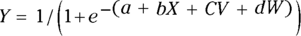
Logistic regression finds the best-fitting values of the parameters a, b, c, and d given your data. That way, for any particular set of values for X, V, and W, you can use the equation to predict Y, which is the probability of being positive for the outcome.
Running a Logistic Regression Model with Software
The theory behind logistic regression is difficult to grasp, and the calculations are complicated (see the sidebar “Getting into the nitty-gritty of logistic regression” for details). The good news is that most statistical software (as described in Chapter 4) can run a logistic regression model, and it is similar to running a straight-line or multiple linear regression model (see Chapters 16 and 17). Here are the steps:
Make sure your data set has a column for the outcome variable that is coded as 1 where the individual is positive for the outcome, and 0 when they are negative.
If you do not have an outcome column coded this way, use the data management commands in your software to generate a new variable coded as 0 for those who do not have the outcome, and 1 for those who have the outcome, as shown in Table 18-1.
Make sure your data set has a column for each predictor variable, and that these columns are coded the way you want them to be entered them into the model.
The predictors can be quantitative, such as age or weight. They can also be categorical, like gender or treatment group. You will need to make decisions about how to recode these variables to enter them into the regression model. See Chapter 17, where we describe how to set up categorical predictor variables.
Tell your software which variables are the predictors and which is the outcome.
Depending on the software, you may do this by typing the variable names, or by selecting the variables from a menu or list.
- Request the optional output from the software if available which may include:
- A summary of information about the variables, goodness-of-fit measures, and a graph of the fitted logistic curve
- A table of regression coefficients, including odds ratios (ORs) and their 95 percent confidence intervals (CIs)
- Predicted probabilities of getting the outcome for each individual, and a classification table of observed outcomes versus predicted outcomes
- Measures of prediction accuracy, which include overall accuracy, sensitivity, and specificity, as well as a Receiver Operator Characteristics (ROC) curve
Execute the model in the software.
Obtain the output you requested, and interpret the resulting model.
Interpreting the Output of Logistic Regression
Figure 18-4 shows two kinds of statistical software output from a logistic regression model produced from the data in Table 18-1. The output presented is not from a particular command in a particular software. Instead, typical output for the different items is presented to enable us to cover many different potential scenarios.

© John Wiley & Sons, Inc.
FIGURE 18-4: Typical output from a logistic regression model. The output on the left (a) shows statistical results output for the model, and the output on the right (b) shows predicted probabilities for each individual that can be output as a data set.
Seeing summary information about the variables
At the top of Figure 18-4a, you can see information about the variables under Descriptives. It can include means and standard deviations of predictors that are numerical variables, and a count of how many individuals did or did not have the outcome event. In Figure 18-4a, you can see that 15 of the 30 individuals lived and 15 died.
Assessing the adequacy of the model
In Figure 18-4a, the middle section starting with Deviance and ending with AIC provides model fit information. These are measures that indicate how well the fitted function represents the data, which is called goodness-of-fit. Some have test statistics and an associated p value (see Chapter 3 for a refresher on p values), while others produce metrics. Although there are different model fit statistics, you will find that they usually agree on how well a model fits the data.
You may see the following model fit measures, depending on your software:
- A p value associated with the decrease in deviance between the null model and the final model: This information is shown in Figure 18-4a under Deviance. Under α = 0.05, if this p value < 0.05, it indicates that adding the predictor variables to the null model statistically significantly improves its ability to predict the outcome. In Figure 18-4a, p < 0.0001, which means that adding radiation dose to the model makes it statistically significantly better at predicting an individual animal’s chance of dying than the null model. However, it’s not very hard for a model with any predictors to be better than the null model, so this is not a very sensitive model fit statistic.
- A p value from the Hosmer-Lemeshow (H-L) test: In Figure 18-4a, this is listed under Hosmer-Lemeshow Goodness of Fit Test. The null hypothesis for this test is your data are consistent with the logistic function’s S shape, so if p < 0.05, your data do not qualify for logistic regression. The focus of the test is to see if the S is getting distorted at very high or very low levels of the predictor (as shown in Figure 18-4b). In Figure 18-4a, the H-L p value is 0.842, which means that the data are consistent with the shape of a logistic curve.
- One or more pseudo–r2values:Pseudo–r2values indicate how much of the total variability in the outcome is explainable by the fitted model. They are analogous to how r2 is interpreted in ordinary least-squares regression, as described in Chapter 17. In Figure 18-4a, two such values are provided under the labels Cox/Snell R-square and Nagelkerke R-square. The Cox/Snell r2 is 0.577, and the Nagelkerke r2 is 0.770, both of which indicate that a majority of the variability in the outcome is explainable by the logistic model.
 Akaike’s Information Criterion (AIC): AIC is a measure of the final model deviance adjusted for how many predictor variables are in the model. Like deviance, the smaller the AIC, the better the fit. The AIC is not very useful on its own, and is instead used for choosing between different models. When all the predictors in one model are nested — or included — in another model with more predictors, the AIC is helpful for comparing these models to see if it is worth adding the extra predictors.
Checking out the table of regression coefficients
Your intention when developing a logistic regression model is to obtain estimates from the table of coefficients, which looks much like the coefficients table from ordinary straight-line or multivariate least-squares regression (see Chapters 16 and 17). In Figure 18-4a, they are listed under Coefficients and Standard Errors. Observe:
- Every predictor variable appears on a separate row.
- There’s one row for the constant term labeled Intercept.
- The first column usually lists the regression coefficients (under Coeff. in Figure 18-4a).
- The second column usually lists the standard error (SE) of each coefficient (under StdErr in Figure 18-4a).
- A p-value column indicates whether the coefficient is statistically significantly different from 0. This column may be labeled Sig or Signif or Pr(> lzl), but in Figure 18-4a, it is labeled p-value.
For each predictor variable, the output should also provide the odds ratio (OR) and its 95 percent confidence interval. These are usually presented in a separate table as they are in Figure 18-4a under Odds Ratios and 95% Confidence Intervals.
Predicting probabilities with the fitted logistic formula
The output may include the fitted logistic formula. At the bottom of Figure 18-4a, the formula is shown as:

You can write out the formula manually by inserting the value of the regression coefficients from the regression table into the logistic formula. The final model produced by the logistic regression program from the data in Table 18-1 and the resulting logistic curve are shown in Figure 18-5.
Once you have the fitted logistic formula, you can predict the probability of having the outcome if you know the value of the predictor variable. For example, if an individual is exposed to 500 REM of radiation, the probability of the outcome is given by this formula: Probability of  , which equals 0.71. An individual exposed to 500 REM of radiation has a predicted probability of 0.71 — or a 71 percent chance — of dying shortly thereafter. The predicted probabilities for each individual are shown in the data listed in Figure 18-4b. You can also calculate some points of special significance on a logistic curve, as you find out in the following sections.
Be careful with your algebra when evaluating these formulas! The a coefficient in a logistic regression is often a negative number, and subtracting a negative number is like adding its absolute value.

© John Wiley & Sons, Inc.
FIGURE 18-5: The logistic curve that fits the data from Table 18-1.
Calculating effective doses on a logistic curve
One point of special significance on a logistic curve with a numerical predictor is a median effective dose. This is a dose (X) that produces a 50 percent response, meaning where  , and is designated ED50. Similarly, the X value that makes
  is called the 80 percent effective dose and is designated ED80, and so on. You can calculate these dose levels from the a and b parameters of the fitted logistic model in the preceding section.
Using your high-school algebra, you can solve the logistic formula 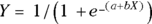 for X as a function of Y. If you don’t remember how to do that, don’t worry, here’s the answer:
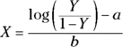
where log stands for natural logarithm. If you substitute 0.5 for Y in the preceding equation because you want to calculate the ED50, the answer is  . Similarly, substituting 0.8 for Y gives the
 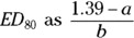 .
.
Imagine a logistic regression model based on a study of participants taking a drug at different doses where the predictor is level of drug dose, and the outcome is that it produces a therapeutic response. The model has  and
and  mg/dL. In this case, the ED80 (or 80 percent effective dose) would be equal to
  , which works out to about 207 mg/dL.
Calculating lethal doses on a logistic curve
When death is the outcome event, the corresponding terms are median lethal dose (abbreviated LD50) and 80 percent lethal dose (abbreviated LD80), and so on. To calculated the LD50 using the data in Table 18-1,  and
and  , so
, so  , which works out to 420 REMs. An LD50 of 420 REMs dose of radiation means an individual has a 50 percent chance of dying shortly after being exposed to this level of radiation.
Making yes or no predictions
If you fit a logistic regression model, then learn of the value of predictor variables for an individual, you can plug them into the equation and calculate the predicted probability of the individual having the outcome. But sometimes, you are trying to actually predict the outcome — whether the event will happen or not, yes or no — to an individual. You can do this by setting a cut value on predicted probability. Imagine you select 0.5 as the cut value, and you make a rule that if the individual’s predicted probability is 0.5 or greater, you’ll predict yes; otherwise, you’ll predict no.
In the following sections, we talk about yes or no predictions. We explain how they expose the ability of the logistic model to make predictions, and how you can strategically select the cut value that gives you the best tradeoff between wrongly predicting yes and wrongly predicting no.
Measuring accuracy, sensitivity, and specificity with classification tables
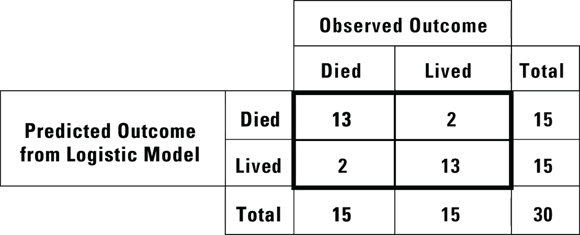
Software output for logistic regression provides several goodness-of-fit measures (see the earlier section “Assessing the adequacy of the model”). One intuitive indicator of goodness-of-fit is the extent to which your yes or no predictions from the logistic model match the actual outcomes. You can cross-tabulate the predicted and observed outcomes into a fourfold classification table. To do this, you would ask the software to generate a classification table for you from the data based on a cut value in the predicted probability. Most software assumes a cut value of 0.5 unless you tell it to use some other value. Figure 18-6 shows the classification table of observed versus predicted outcomes from radiation exposure, using a cut value of 0.5 predicted probability.
From the classification table shown in Figure 18-6, you can calculate several useful measures of the model’s predicting ability for any specified cut value, including the following:
© John Wiley & Sons, Inc.
FIGURE 18-6: The classification table for the radiation example.
- Overall accuracy: This refers to the proportion of accurate predictions, as shown in the concordant cells, which are the upper-left and lower-right. Of the 30 individuals in the data set from Table 18-1, the logistic model predicted correctly
 = 0.87, or about 87 percent of the time. This means with the cut value where you placed it, the model would make a wrong prediction only about 13 percent of the time.
 - Sensitivity: This refers to the proportion of yes outcomes predicted accurately. As seen in the upper-left cell in Figure 18-6, with the cut value where it was placed, the logistic model predicted 13 of the 15 observed deaths (yes outcomes). So the sensitivity is
 = 0.87, or about 87 percent. This means the model would have a false-negative rate of 13 percent.
 - Specificity: This refers to the proportion of no outcomes predicted accurately. In the lower-right cell of Figure 18-6, the model predicted survival in 13 of the 15 observed survivors. So, the specificity is
 = 0.87, or about 87 percent. This means the model would have a false-positive rate of 13 percent.
Sensitivity and specificity are especially relevant to screening tests for diseases. An ideal test would have 100 percent sensitivity and 100 percent specificity, and therefore, 100 percent overall accuracy. In reality, no test could meet these standards, and there is a tradeoff between sensitivity and specificity.
By judiciously choosing the cut value for converting a predicted probability into a yes or no decision, you can often achieve high sensitivity or high specificity, but it’s hard to maximize both simultaneously. Screening tests are meant to detect disease, so how you select the cut value depends upon what happens if it produces a false-positive or false-negative result. This helps you decide whether to prioritize sensitivity or specificity.
The sensitivity and specificity of a logistic model depends upon the cut value you set for the predicted probability. The trick is to select a cut value that gives the optimal combination of sensitivity and specificity, striking the best balance between false-positive and false-negative predictions, in light of the different consequences of the two types of false predictions. A false-positive screening result from a mammogram may mean the patient is worried until the negative diagnosis is confirmed by ultrasound, and a false-negative screening results from a prostate cancer screening may result in a delay in identifying the prostate tumor. To find this optimal cut value, you need to know precisely how sensitivity and specificity play against each other — that is, how they simultaneously vary with different cut values. There’s a neat way to do that which we explain in the following section.
Rocking with ROC curves
The graph used to display the sensitivity/specificity tradeoff for any fitted logistic model is called the Receiver Operator Characteristics (ROC) graph. The name comes from its original use during World War II to analyze the performance characteristics of people who operated RADAR receivers, but the name has stuck, and now it is also referred to as an ROC curve.
An ROC graph has a curve that shows you the complete range of sensitivity and specificity that can be achieved for any fitted logistic model based on the selected cut value. The software generates an ROC curve by effectively trying all possible cut values of predicted probability between 0 and 1, calculating the predicted outcomes, cross-tabbing them against the observed outcomes, calculating sensitivity and specificity, and then graphing sensitivity versus specificity. Figure 18-7 shows the ROC curve from the logistic model developed from the data in Figure 18-1 (using R software; see Chapter 4).

© John Wiley & Sons, Inc.
FIGURE 18-7: ROC curve from dose mortality data.
As shown in Figure 18-7, the ROC curve always starts in the lower-left corner of the graph, where 0 percent sensitivity intersects with 100 percent specificity. It ends in the upper-right corner, where 100 percent sensitivity intersects with 0 percent specificity. Most software also draws a diagonal straight line between the lower-left and upper-right corners because that represents the formula:  . If your model’s ROC curve were to match that line, it would indicate the total absence of any predicting ability at all of your model.
Like Figure 18-7, every ROC graph has sensitivity running up the Y axis, which is displayed either as fractions between 0 and 1 or as percentages between 0 and 100. The X axis is either presented from left to right as 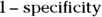 , or like it is in Figure 18-7, where specificity is labeled backwards — from right to left — along the X axis.
Most ROC curves lie in the upper-left part of the graph area. The farther away from the diagonal line they are, the better the predictive model is. For a nearly perfect model, the ROC curve runs up along the Y axis from the lower-left corner to the upper-left corner, then along the top of the graph from the upper-left corner to the upper-right corner.
Because of how sensitivity and specificity are calculated, the graph appears as a series of steps. If you have a large data set, your graph will have more and smaller steps. For clarity, we show the cut values for predicted probability as a scale along the ROC curve itself in Figure 18-7, but unfortunately, most statistical software doesn’t do this for you.
Looking at the ROC curve helps you choose a cut value that gives the best tradeoff between sensitivity and specificity:
- To have very few false positives: Choose a higher cut value to give a high specificity. Figure 18-7 shows that by setting the cut value to 0.6, you can simultaneously achieve about 93 percent specificity and 87 percent sensitivity.
- To have very few false negatives: Choose a lower cut value to give higher sensitivity. Figure 18-7 shows you that if you set the cut value to 0.3, you can have almost perfect sensitivity because you’ll be at almost 100 percent, but your specificity will be only about 75 percent, meaning you’ll have a 25 percent false positive rate.
The software may optionally display the area under the ROC curve (abbreviated AUC), along with its standard error and a p value. This is another measure of how good the predictive model is. The diagonal line has an AUC of 0.5, and there is a statistical test comparing your AUC to the diagonal line. Under α = 0.05, if the p value < 0.05, it indicates that your model is statistically significantly better than the diagonal line at accurately predicting your outcome.
Heads Up: Knowing What Can Go Wrong with Logistic Regression
Logistic regression presents many of the same potential pitfalls as ordinary least-squares regression (see Chapters 16 and 17), as well as several that are specific to logistic regression. Watch out for some of the more common pitfalls:
- Don’t fit a logistic function to non-logistic data: Don’t use logistic regression to fit data that doesn’t behave like the logistic S curve. Plot your grouped data (as shown earlier in Figure 18-1b), and if it’s clear that the fraction of positive outcomes isn’t leveling off at
 or
or  for very large or very small X values, then logistic regression is not the correct modeling approach. The H-L test described earlier under the section “Assessing the adequacy of the model” provides a statistical test to determine if your data qualify for logistic regression. Also, in Chapter 19, we describe a more generalized logistic model that contains other parameters for the upper and lower leveling-off values.
 - Watch out for collinearity and disappearing significance: When you are doing any kind of regression and two or more predictor variables are strongly related with each other, you can be plagued with problems of collinearity. We describe this problem in Chapter 17, and potential modeling solutions in Chapter 20.
- Check for inadvertent reverse-coding of the outcome variable: The outcome variable should always be coded as 1 for a yes outcome and 0 for a no outcome (refer to Table 18-1 for an example). If the variable in the data set is coded using characters, you should recode an outcome variable using the 0/1 coding. It is important you do the coding yourself, and do not leave it to an automated function in the program, because it may inadvertently reverse the coding so that 1 = no and 0 = yes. This error of reversal won’t affect any p values, but it will cause all your ORs and their CIs to be the reciprocals of what they would have been, meaning they will refer to the odds of no rather than the odds of yes.
- Don’t misinterpret odds ratios for categorical predicators: Categorical predictors should be coded numerically as we describe in Chapter 8. It is important to ensure that proper indicator variable coding is used, and these variables are introduced properly in the model, as described in Chapter 17.
Also, be careful not to misinterpret odds ratios for numerical predictors, and be mindful of the complete separation problem, as described in the following sections.
Don’t misinterpret odds ratios for numerical predictors
The OR always represents the factor by which the odds of getting the outcome event increases when the predictor increases by exactly one unit of measure, whatever that unit may be. Sometimes you may want to express the OR in more convenient units than what the data was recorded in. For the example in Table 18-1, the OR for dose as a predictor of death is 1.0115 per REM. This isn’t too meaningful because one REM is a very small increment of radiation. By raising 1.0115 to the 100th power, you get the equivalent OR of 3.1375 per 100 REMs, and you can express this as, “Every additional 100 REMs of radiation more than triples the odds of dying.”
The value of a regression coefficient depends on the units in which the corresponding predictor variable is expressed. So the coefficient of a height variable expressed in meters is 100 times larger than the coefficient of height expressed in centimeters. In logistic regression, ORs are obtained by exponentiating the coefficients, so switching from centimeters to meters corresponds to raising the OR (and its confidence limits) to the 100th power.
Beware of the complete separation problem
Imagine your logistic regression model perfectly predicted the outcome, in that every individual positive for the outcome had a predicted probability of 1.0, and every individual negative for the outcome had a 0 predicted probability. This is called perfect separation or complete separation, and the problem is called the perfect predictor problem. This is a nasty and surprisingly frequent problem that’s unique to logistic regression, which highlights the sad fact that a logistic regression model will fail to converge in the software if the model fits perfectly!
If the predictor variable or variables in your model completely separate the yes outcomes from the no outcomes, the maximum likelihood method will try to make the coefficient of that variable infinite, which usually causes an error in the software. If the coefficient is positive, the OR tries to be infinity, and if it is negative, it tries to be 0. The SE of the OR tries to be infinite, too. This may cause your CI to have a lower limit of 0, an upper limit of infinity, or both.
Check out Figure 18-8, which visually describes the problem. The regression is trying to make the curve come as close as possible to all the data points. Usually it has to strike a compromise, because there’s a mixture of 1s and 0s, especially in the middle of the data. But with perfectly separated data, no compromise is necessary. As b becomes infinitely large, the logistic function morphs into a step function that touches all the data points (observe where b = 5).
While it is relatively easy to identify if there is a perfect predictor in your data set by looking at frequencies, you may run into the perfect predictor problem as a result of a combination of predictors in your model. Unfortunately, there aren’t any great solutions to this problem. One proposed solution called the Firth correction allows you to add a small number roughly equivalent to half an observation to the data set that will disrupt the complete separation. If you can do this correction in your software, it will produce output, but the results will likely be unstable (very near 0, or very near infinity). The approach of trying to fix the model by changing the predictors would not make sense, since the model fits perfectly. You may be forced to abandon your logistic regression plans and instead provide a descriptive analysis.

© John Wiley & Sons, Inc.
FIGURE 18-8: Visualizing the complete separation (or perfect predictor) problem in logistic regression.
Figuring Out the Sample Size You Need for Logistic Regression
Estimating the required sample size for a logistic regression can be a pain, even for a simple one-predictor model. You will have no problem specifying desired power and α level (see Chapter 3 for more about these items). And, you can state the effect size of importance as an OR.
Assuming a one-predictor model, the required sample size for logistic regression also depends on the relative frequency of yes and no outcomes, and how the predictor variable is distributed. And with multiple predictors in the model, determining sample size is even more complicated. So for a rigorous sample-size calculation for a study that will use a logistic regression model with multiple predictors, you may have no choice but to seek the help of a professional statistician.
Here are two simple approaches you can use if your logistic model has only one predictor. In each case, you replace the logistic regression equation with another equation that is somewhat equivalent, and then do a sample-size calculation based on that. It’s not an ideal solution, but it can give you an answer that’s close enough for planning purposes.
- If the predictor is a dichotomous category (a yes/no variable), logistic regression gives the same p value you get from analyzing a fourfold table. Therefore, you can use the sample-size calculations we describe in Chapter 12.
- If the predictor is a continuous numerical quantity (like age), you can pretend that the outcome variable is the predictor, and age is the outcome. We realize this flips the cause-and-effect relationship backwards, but if you allow that conceptual flip, then you can ask whether the two different outcome groups have different mean values for the predictor. You can test that question with an unpaired Student t test, so you can use the sample-size calculations we describe in Chapter 11.