Chapter 12
Comparing Proportions and Analyzing Cross-Tabulations
IN THIS CHAPTER
 Testing for association between categorical variables with the Pearson chi-square and Fisher Exact tests
Estimating sample sizes for tests of association
Suppose that you are studying pain relief in patients with chronic arthritis. Some are taking nonsteroidal anti-inflammatory drugs (NSAIDs), which are over-the-counter pain medications. But others are trying cannabidiol (CBD), a new potential natural treatment for arthritis pain. You enroll 100 chronic arthritis patients in your study and you find that 60 participants are using CBD, while the other 40 are using NSAIDs. You survey them to see if they get adequate pain relief. Then you record what each participant says (pain relief or no pain relief). Your data file has two dichotomous categorical variables: the treatment group (CBD or NSAIDs), and the outcome (pain relief or no pain relief).
You find that 10 of the 40 participants taking NSAIDs reported pain relief, which is 25 percent. But 33 of the 60 taking CBD reported pain relief, which is 55 percent. CBD appears to increase the percentage of participants experiencing pain relief by 30 percentage points. But can you be sure this isn’t just a random sampling fluctuation?
Data from two potentially associated categorical variables is summarized as a cross-tabulation, which is also called a cross-tab or a two-way table. Because we are studying the association between two variables, this is a form of bivariate analysis. The rows of the cross-tab represent the different categories (or levels) of one variable, and the columns represent the different levels of the other variable. The cells of the table contain the count of the number of participants with the indicated levels for the row and column variables. If one variable can be thought of as the “cause” or “predictor” of the other, the cause variable becomes the rows, and the “outcome” or “effect” variable becomes the columns. If the cause and outcome variables are both dichotomous, meaning they have only two levels (like in this example), then the cross-tab has two rows and two columns. This structure contains four cells containing counts, and is referred to as a 2-by-2 (or 2 × 2) cross-tab, or a fourfold table. Cross-tabs are displayed with an extra row at the bottom and an extra column at the right to contain the sums of the cells in the rows and columns of the table. These sums are called marginal totals, or just marginals.
Comparing proportions based on a fourfold table is the simplest example of testing the association between two categorical variables. More generally, the variables can have any number of categories, so the cross-tab can be larger than 2 × 2, with multiple rows and many columns. But the basic question to be answered is always the same: Is the spread of numbers across the columns so different from one row to the next that the numbers can’t be explained away as random fluctuations? Another way of asking the same question is: Is being a member of a particular row associated with being a member of a particular column?
In this chapter, we describe two tests you can use to answer this question: the Pearson chi-square test, and the Fisher Exact test. We also explain how to estimate power and sample sizes for the chi-square and Fisher Exact tests.
 Like with other statistical tests, you can run all the tests in this chapter from individual-level data in a database, where there is one record per participant. But the tests in this chapter can also be executed using data that has already been summarized in the form of a cross-tab:
- Most statistical software is set up to work with individual-level data. In that case, your data file needs to have two columns for the association you want to test: one containing the categorical variable representing the treatment group (or whatever category is on the y-axis), and one containing the categorical variable representing the outcome. If you have the correct columns, all you have to do is tell the statistical software you are using which test or tests you want to run, and which variables to use in the test.
- Most statistical software is also set up so that you can do these tests using summarized data (rather than individual-level data), so long as you set an option in your programming when running the tests. In contrast, online calculators that execute these tests expect you to have already cross-tabulated the data. These calculators usually present a screen showing an empty table, and you enter the counts into the table’s cells to run the calculation.
Examining Two Variables with the Pearson Chi-Square Test
The most commonly used statistical test of association between two categorical variables is called the chi-square test of association developed by Karl Pearson around the year 1900. It’s called the chi-square test because it involves calculating a number called a test statistic that fluctuates in accordance with the chi-square distribution. Many other statistical tests also use the chi-square distribution, but the test of association is by far the most popular. In this book, whenever we refer to a chi-square test without specifying which one, we are referring to the Pearson chi-square test of association between two categorical variables. (Please note that some books use the notation X2 or x2 instead of saying the term chi-square.)
Understanding how the chi-square test works
You don’t have to understand the equations behind the chi-square test if you have a computer to do them, which is optimal, though it is possible to calculate the test manually. This means you technically don’t have to read this section. But we encourage you to do so anyway, because we think you’ll have a better appreciation for the strengths and limitations of the test if you know its mathematical underpinnings. Here, we walk you through conducting a chi-square test manually (which is possible to do in Microsoft Excel).
Calculating observed and expected counts
All statistical significance tests start with a null hypothesis ( ) that asserts that no real effect is present in the population, and any effect you think you see in your sample is due only to random fluctuations. (See Chapter 3 for more information.) The
  for the chi-square test asserts that there’s no association between the levels of the row variable and the levels of the column variable, so you should expect the relative spread of cell counts across the columns to be the same for each row.
Figure 12-1 shows how this works out for the observed data taken from the example in this chapter’s introduction. You can see from the marginal “Total” row that the overall rate of pain relief (for both groups combined) is 43/100, or 43 percent.

© John Wiley & Sons, Inc.
FIGURE 12-1: The observed results comparing CBD to NSAIDs for the treatment of pain from chronic arthritis.
Figure 12-1 presents the actual data you observed from your survey, where the observed counts are placed in each of the four cells. As part of the chi-square test statistic calculation, you now need to calculate an expected count for each cell. This is done by taking the product of the row and column marginals and dividing them by the total. So, to determine the expected count in the CBD/pain relief cell, you would multiply 43 (row marginal) by 60 (column marginal), then divide this by 100 (total) which comes out 25.8. Figure 12-2 presents the fourfold table with the expected counts in the cells.

© John Wiley & Sons, Inc.
FIGURE 12-2: Expected cell counts if the null hypothesis is true (there is no association between either drug and the outcome).
The reason you need these expected counts is that they represent what would happen under the null hypothesis (meaning if the null hypothesis were true). If the null hypothesis were true:
- In the CBD-treated group, you’d expect about 25.8 participants to experience pain relief (43 percent of 60), with the remaining 34.2 reporting no pain relief.
- In the NSAIDs-treated group, you’d expect about 17.2 participants to feel pain relief (43 percent of 40) with the remaining 22.8 reporting no pain relief.
As you can see, this expected table assumes that you still have the overall pain relief rate of 43 percent, but that you also have the pain relief rates in each group equal to 43 percent. This is what would happen under the null hypothesis.
Now that you have observed and expected counts, you’re no doubt curious as to how each cell in the observed table differs from its companion cell in the expected table. To get these numbers, you can subtract each expected count from the observed count in each cell to get a difference table (observed – expected), as shown in Figure 12-3.

© John Wiley & Sons, Inc.
FIGURE 12-3: Differences between observed and expected cell counts if the null hypothesis is true.
As you review Figure 12-3, because you know the observed and expected tables in Figures 12-1 and 12-2 always have the same marginal totals by design, you should not be surprised to observe that the marginal totals in the difference table are all equal to zero. All four cells in the center of this difference table have the same absolute value (7.2), with a plus and a minus value in each row and each column.
The pattern just described is always the case for  tables. For larger tables, the difference numbers aren’t all the same, but they always sum up to zero for each row and each column.
The values in the difference table in Figure 12-3 show how far off from  your observed data are. The question remains: Are those difference values larger than what may have arisen from random fluctuations alone if
  is really true? You need some kind of measurement unit by which to judge how unlikely those difference values are. Recall from Chapter 10 that the standard error (SE) expresses the general magnitude of random sampling, so looking at the SE as a type of measurement unit is a good way for judging the size of the differences you may expect to see from random fluctuations alone. It turns out that it is easy to approximate the SE of the differences because this is approximately equal to the square root of the expected counts. The rigorous proof behind this is too complicated for most mathophobes (as well as some normal people) to understand. Nevertheless, a simple informal explanation is based on the idea that random event occurrences typically follow the Poisson distribution for which the SE of the event count equals the square root of the expected count (as discussed in Chapter 10).
Summarizing and combining scaled differences
For the upper-left cell in the cross-tab (CBD–treated participants who experience pain relief), you see the following:
- The observed count (Ob) is 33.
- The expected count (Ex) is 25.8.
- The difference (Diff) is
 , or
, or  .
. - The SE of the difference is
 or
or 
You can “scale” the Ob-Ex difference (in terms of unit of SE) by dividing it by the SE measurement unit, getting the ratio  , or 1.42. This means that the difference between the observed number of CBD-treated participants who experience pain relief and the number you would have expected if the CBD had no effect on survival is about 1.42 times as large as you would have expected from random sampling fluctuations alone. You can do the same calculation for the other three cells and summarize these scaled differences. Figure 12-4 shows the differences between observed and expected cell counts, scaled according to the estimated standard errors of the differences.

© John Wiley & Sons, Inc.
FIGURE 12-4: Differences between observed and expected cell counts.
The next step is to combine these individual scaled differences into an overall measure of the difference between what you observed and what you would have expected if the CBD or NSAID use really did not impact pain relief differentially. You can’t just add them up because the negative and positive differences would cancel each other out. You want all differences (positive and negative) to contribute to the overall measure of how far your observations are from what you expected under  .
.
Instead of summing the differences, statisticians prefer to sum the squares of differences, because the squares are always positive. This is exactly what’s done in the chi-square test. Figure 12-5 shows the squared scaled differences, which are calculated from the observed and expected counts in Figures 12-1 and 12-2 using the formula  (rather than by squaring the rounded-off numbers in Figure 12-4, which would be less accurate).

© John Wiley & Sons, Inc.
FIGURE 12-5: Components of the chi-square statistic: squares of the scaled differences.
You then add up these squared scaled differences:  to get the chi-square test statistic. This sum is an excellent test statistic to measure the overall departure of your data from the null hypothesis:
- If the null hypothesis is true (use of CBD or NSAID does not impact pain relief status), this statistic should be quite small.
- If one of the levels of treatment has a disproportionate association with the outcome (in either direction), it will affect the whole table, and the result will be a larger test statistic.
Determining the p value
Now that you calculated the test statistic, the only remaining task before interpretation is to determine the p value. The p value represents the probability that random fluctuations alone, in the absence of any true effect of CBD or NSAIDs on pain relief, could lead to a value of 8.81 or greater for this test statistic. (We introduce p values in Chapter 3.) Once again, the rigorous proof is very complicated, so we present an informal explanation:
When the expected cell counts are very large, the Poisson distribution becomes very close to a normal distribution (see Chapter 24 for more on the Poisson distribution). If the  is true, each scaled difference should be an approximately normally distributed random variable with a mean of zero and a standard deviation of 1. The mean is zero because you subtract the expected value from the observed value, and the standard deviation is 1 because it is divided by the SE. The sum of the squares of one or more normally distributed random numbers is a number that follows the chi-square distribution (also covered in Chapter 24). So the test statistic from this test should follow the chi-square distribution. Now it is obvious why it is named the chi-square test! The next step is to obtain the p value for the test statistic. To do that manually, you would look up the test statistic (which is 8.81 in our case) in a chi-square table.
In actuality, the chi-square distribution refers to a family of distributions. Which chi-square distribution you are using depends upon a number called the degrees of freedom, abbreviated d.f. or df or by the Greek lowercase letter nu (v) (in this book we use df). The df is a measure of the probability of independence between the value of the predictor (row) variable and value of the column (outcome) variable.
How would you calculate the df for a chi-square test? The answer is it depends on the number of rows in the cross-tab. For the  cross-tab (fourfold table) in this example, you added up the four values in Figure 12-5, so you may think that you should look up the 8.81 chi-square value with 4 df. But you’d be wrong. Note the italicized word independence in the preceding paragraph. And keep in mind that the differences (
 ) in any row or column always add up to zero. The four terms making up the 8.81 total aren’t independent of each other. It turns out that the chi-square test statistic for a fourfold table has only 1 df, not 4. In general, an N-by-M table, with N rows, M columns, and therefore
  cells, has only
 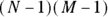 df because of the constraints on the row and column sums. In our case, N — which is the number of rows — is 2, so N-1 is 1. Also, M — which is the number of columns — is 2, so M-1 is 1 also (and 1 times 1 is 1). Don’t feel bad if this wrinkle caught you by surprise — even Karl Pearson who invented the chi-square test got that part wrong!
So, if you were to manually look up the chi-square test statistic of 8.81 in a chi-square table, you would have to look under the distribution for 1 df to find out the p value. Alternatively, if you got this far and you wanted to use the statistical software R to look up the p value, you would use the following code: pchisq(8.81, 1, lower.tail = FALSE). Either way, the p value for chi-square = 8.81, with 1 df, is 0.003. This means that there’s only a 0.003 probability that random fluctuations could produce the effect seen, where CBD performs so differently than NSAIDs with respect to pain relief in chronic arthritis patients. A 0.003 probability is the same as 1 chance in 333 (because  ), meaning very unlikely, but not impossible. So, if you set α = 0.05, because 0.003 < 0.05, your conclusion would be that in the chronic arthritis patients in our sample, whether the participant took CBD or NSAIDs was statistically significantly associated with whether or not they felt pain relief.
Putting it all together with some notation and formulas
 The calculations of the Pearson chi-square test can be summarized concisely using the cell-naming conventions shown in Figure 12-6, along with the standard summation notation described in Chapter 2.

© John Wiley & Sons, Inc.
FIGURE 12-6: A general way of naming the cells of a cross-tab table.
Using these conventions, the basic formulas for the Pearson chi-square test are as follows:
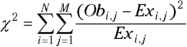
- Expected values:
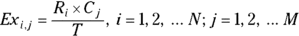
- Chi-square statistic:
- Degrees of freedom:
where i and j are array indices that indicate the row and column, respectively, of each cell.
Pointing out the pros and cons of the chi-square test
The Pearson chi-square test is very popular for several reasons:
- It’s easy! The calculations are simple to do manually in Microsoft Excel (although this is not recommended because the risk of making a typing mistake is high). As described earlier, statistical software packages like the ones discussed in Chapter 4 can perform the chi-square test for both individual-level data as well as summarized cross-tabulated data. Also, several websites can perform the test, and the test has been implemented on smartphones and tablets.
- It’s flexible! The test works for tables with any number of rows and columns, and it easily handles cell counts of any magnitude. Statistical software can usually complete the calculations quickly, even on big data sets.
 But the chi-square test has some shortcomings:
- It’s not an exact test. The p value it produces is only approximate, so using
 as your criterion for statistical significance (meaning setting α = 0.05) doesn’t necessarily guarantee that your Type I error rate will be only 5 percent. Remember, your Type I error rate is the likelihood you will claim statistical significance on a difference that is not true (see Chapter 3 for an introduction to Type I errors). The level of accuracy of the statistical significance is high when all the cells in the table have large counts, but it becomes unreliable when one or more cell counts is very small (or zero). There are different recommendations as to the minimum counts you need per cell in order to confidently use the chi-square test. A rule of thumb that many analysts use is that you should have at least five observations in each cell of your table (or better yet, at least five expected counts in each cell).
 - It’s not good at detecting trends. The chi-square test isn’t good at detecting small but steady progressive trends across the successive categories of an ordinal variable (see Chapter 4 if you’re not sure what ordinal is). It may give a significant result if the trend is strong enough, but it’s not designed specifically to work with ordinal categorical data. In those cases, you should use a Mantel-Haenszel chi-square test for trend, which is outside the scope of this book.
Modifying the chi-square test: The Yates continuity correction
There is a little drama around the original Pearson chi-square of association test that needs to be mentioned here. Yates, who was a contemporary of Pearson, developed what is called the Yates continuity correction. Yates argued that in the special case of the fourfold table, adding this correction results in more reliable p values. The correction consists of subtracting 0.5 from the magnitude of the ( ) difference before squaring it.
Let’s apply the Yates continuity correction for your analysis of the sample data in the earlier section “Understanding how the chi-square test works.” Take a look at Figure 12-3, which has the differences between the values in the observed and expected cells. The application of the Yates correction changes the 7.20 (or –7.20) difference in each cell to 6.70 (or –6.70). This lowers the chi-square value from 8.81 down to 7.63 and increases the p value from 0.0030 to 0.0057, which is still very significant — the chance of random fluctuations producing such an apparent effect in your sample is only about 1 in 175 (because  ).
).
 Even though the Yates correction to the Pearson chi-square test is only applicable to the fourfold table (and not tables with more rows or columns), some statisticians feel the Yates correction is too strict. Nevertheless, it has been automatically built into statistical software like R, so if you run a Pearson chi-square using most commercial software, it automatically uses the Yates correction when analyzing a fourfold table (see Chapter 4 for a discussion of statistical software).
Focusing on the Fisher Exact Test
The Pearson chi-square test described earlier isn’t the only way to analyze cross-tabulated data. Remember that one of the cons was that it is not an exact test? Famous but controversial statistician R. A. Fisher invented another test in the 1920s that gives the exact p value for tables that can handle very small cell counts (even cell counts of zero!). Not surprisingly, this test is called the Fisher Exact test (also sometimes referred to Fisher’s exact test, or just Fisher).
Understanding how the Fisher Exact test works
Like with the chi-square, you don’t have to know the details of the Fisher Exact test to use it. If you have a computer do the calculations for you (which we always recommend), you technically don’t have to read this section. But we encourage you to read this section anyway so you’ll have a better appreciation for the strengths and limitations of this test.
This test is conceptually pretty simple. Instead of taking the product of the marginals and dividing it by the total for each cell as is done with the chi-square test statistic, Fisher exact test looks at every possible table that has the same marginal totals as your observed table. You calculate the exact probability (Pr) of getting each individual table using a formula that, for a fourfold table (using the notation for Figure 12-6), is
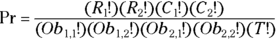
Those exclamation points indicate calculating the factorials of the cell counts (see Chapter 2). For the example in Figure 12-1, the observed table has a probability of
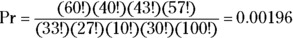
Other possible tables with the same marginal totals as the observed table have their own Pr values, which may be larger than, smaller than, or equal to the Pr value of the observed table. The Pr values for all possible tables with a specified set of marginal totals always add up to exactly 1.
The Fisher Exact test p value is obtained by adding up the Pr values for all tables that are at least as different from the  as your observed table. For a fourfold table that means adding up all the Pr values that are less than (or equal to) the Pr value for your observed table.
For the example in Figure 12-1, the p value comes out to 0.00385, which means that there’s only 1 chance in 260 (because  ) that random fluctuations could have produced such an apparent effect in your sample.
Noting the pros and cons of the Fisher Exact test
The big advantages of the Fisher Exact test are as follows:
- It gives the exact p value.
- It is exact for all tables, with large or small (or even zero) cell counts.
Why do people still use the chi-square test, which is approximate and doesn’t work for tables with small cell counts? Well, there are several problems with the Fisher Exact test:
- The Fisher calculations are a lot more complicated, especially for tables larger than
 . Many statistical software packages either don’t offer the Fisher Exact test or offer it only for fourfold tables. Even if they offer it, you may execute the test and find that it fails to finish the test, and you have to break into the program to stop the procedure. Also, some interactive web pages perform the Fisher Exact test for fourfold tables (including
 www.socscistatistics.com/tests/fisher/default2.aspx). Only the major statistical software packages (like SAS, SPSS, and R, described in Chapter 4) offer the Fisher Exact test for tables larger than because the calculations are so intense. For this reason, the Fisher Exact test is only practical for small cell counts.
 - The calculations can become numerically unstable for large cell counts, even in a
 table. The equations involve the factorials of the cell counts and marginal totals, and these can get very large — even for modest sample sizes — often exceeding the largest number that a computer program can handle. Many programs and web pages that offer the Fisher Exact test for fourfold tables fail with data from more than 100 subjects.
 - Another issue is — like the chi-square test — the Fisher Exact test is not for detecting gradual trends across ordinal categories.
Calculating Power and Sample Size for Chi-Square and Fisher Exact Tests
Note: The basic ideas of power and sample-size calculations are described in Chapter 3, and you should review that information before going further here.
Earlier in the section “Examining Two Variables with the Pearson Chi-Square Test,” we used an example of an observational study design in which study participants were patients who chose which treatment they were using. In this section, we use an example from a clinical trial study design in which study participants are assigned to a treatment group. The point is that the tests in this section work on all types of study designs.
Let’s calculate sample size together. Suppose that you’re planning a study to test whether giving a certain dietary supplement to a pregnant woman reduces her chances of developing morning sickness during the first trimester of pregnancy, which is the first three months. This condition normally occurs in 80 percent of pregnant women, and if the supplement can reduce that incidence rate to only 60 percent, it would be considered a large enough reduction to be clinically significant. So, you plan to enroll a group of pregnant women who are early in their first trimester and randomize them to receive either the dietary supplement or a placebo that looks, smells, and tastes exactly like the supplement. You will randomly assign each participant to the either the supplement group or the placebo group in a process called randomization. The participants will not be told which group they are in, which is called blinding. (There is nothing unethical about this situation because all participants will agree before participating in the study that they would be willing to take the product associated with each randomized group, regardless of the one to which they are randomized.)
You’ll have them take the product during their first trimester, and you’ll survey them to record whether they experience morning sickness during that time (using explicit criteria for what constitutes morning sickness). Then you’ll tabulate the results in a 2 × 2 cross-tab. The table will look similar to Figure 12-1, but instead will say “supplement” and “placebo” as the label on the two rows, and “did” and “did not” experience morning sickness as the headings on the two columns. And you’ll test for a significant effect with a chi-square or Fisher Exact test. So, your sample size calculation question is: How many subjects must you enroll to have at least an 80 percent chance of getting on the test if the supplement truly can reduce the incidence from 80 percent to 60 percent?
You have several ways to estimate the required sample size. The most general and most accurate way is to use power/sample-size software such as G*Power, which is described in detail in Chapter 4. Or you can use the online sample-size calculator at https://clincalc.com/stats/samplesize.aspx, which produces the same results.
You need to enroll additional subjects to allow for possible attrition during the study. If you expect x percent of the subjects to drop out, your enrollment should be:

So, if you expect 15 percent of enrolled subjects to drop out and therefore be unanalyzable, you need to enroll 100 × 197/(100 – 15), or about 231 participants.