Chapter 7
Having Designs on Study Design
IN THIS CHAPTER
 Grasping the hierarchy of study designs in epidemiology
Appreciating relative strength of different study designs for causal inference
Getting the details about different study designs
Biostatistics can be seen as the application of a set of tools to answer questions posed through human research. When studying samples, these tools are used in conjunction with epidemiologic study designs in such a way as to facilitate causal inference, or the ability to determine cause and effect. Some study designs are better than others at facilitating causal inference. Nevertheless, regardless of the study design selected, an appropriate sampling strategy and statistical analysis that complements the study design must be used in conjunction with it.
In this chapter, we provide an overview of epidemiologic study designs and present them in a hierarchy so that you can relate them to the biostatistical approaches described in the different chapters of this book. We start by looking at broad study design categories such as observational, experimental, descriptive, and analytic, and move into descriptive study designs including expert opinion, case studies and case series, ecological (correlational) studies, and cross-sectional studies. We present analytic study designs next — case-control studies and longitudinal cohort studies — which are superior to descriptive designs in terms of developing evidence for causal inference, and then move into the highest-level designs: systematic reviews and meta-analyses.
 For a deeper dive into epidemiologic study designs, we encourage you to read Epidemiology For Dummies by Amal K. Mitra (Wiley) and pay special attention to Chapters 16 and 17, which are about causal inference and study design.
Presenting the Study Design Hierarchy
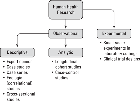
Figure 7-1 illustrates the epidemiologic study designs in terms of their relationship with each other in a hierarchy as they apply to human health research (not animal research or other domains of human research like psychology). As shown in Figure 7-1, human health research may be split into two types: observational and experimental.
© John Wiley & Sons, Inc.
FIGURE 7-1: Study design hierarchy.
Observational research is where humans are studied in terms of their health and behavior, but they are not assigned to do any particular behavior as part of the study — they are just observed. For example, imagine that a sample of women were contacted by phone and asked about their use of birth control pills. In this case, researchers are observing their behavior with regard to birth control pills.
This is in contrast to experimental research, which is where the researcher assigns research participants to engage in certain behaviors as part of an intervention being studied. Imagine that you were studying a new birth control pill on the market and you wanted to know whether taking it changed a woman’s lipid profile, which is determined by a laboratory test. You may do an experiment where you assign research participants to take the pill and then evaluate their lipid profiles.
 The difference between observational and experimental research is important because there is a heavier ethical obligation in experimental research when the researcher is assigning an intervention. Also, because of such ethical considerations in addition to time, cost, and other limitations, there are far more observational studies than experimental studies.
Note that there are only two entries under the experimental category in Figure 7-1 — small-scale experiments in laboratory settings and clinical trial designs. The example of assigning research participants to take a new birth control pill and then testing their lipid profiles is an example of a small-scale experiment in a laboratory setting. We describe clinical trials later in this chapter in “Advancing to the clinical trial stage.”
Observational studies, on the other hand, can be further subdivided into two types: descriptive and analytic. Descriptive study designs include expert opinion, case studies, case series, ecologic (correlational) studies, and cross-sectional studies. These designs are called descriptive study designs because they focus on describing health in populations. (We explain what this means in “Describing What We See.”) In contrast to descriptive study designs, there are only two types of analytic study designs: longitudinal cohort studies and case-control studies. Unlike descriptive studies, analytic studies are designed specifically for causal inference. These are described in more detail in the section, “Getting Analytical.”
Describing what we see
As shown in Figure 7-1, there are two types of observational studies: descriptive and analytic. Descriptive study designs focus on describing patterns of human health and disease in populations, usually as part of surveillance, which is the act of quantifying patterns of health and disease in populations. Cross-sectional is one descriptive study design used in surveillance to produce incidence and prevalence rates of conditions or behaviors (see Chapter 14). For example, results from cross-sectional surveillance studies tell us that approximately 25 percent of women aged 15 to 44 who currently use contraception in the United States choose the birth control pill as their method of choice. While descriptive study designs are necessary in a practical sense, they are poor at developing evidence for causal inference, so they are considered inferior to analytic study designs.
Getting analytical
Analytic designs include longitudinal cohort studies and case-control studies. These are the strongest observational study designs for causal inference. Longitudinal cohort studies are used to study causes of more common conditions, like hypertension (HTN). It is called longitudinal because follow-up data are collected over years to see which members of the sample, or cohort, eventually get the outcome, and which members do not. (In a cohort study, none of the participants has the condition, or outcome, when they enter the study.) The cohort study design is described in more detail under the section, “Following a cohort over time.”
Case-control studies are used when the outcome is not that common, such as liver cancer. In the case of rare conditions, first a group of individuals known to have the rare condition (cases) is identified and enrolled in the study. Then, a comparable group of individuals known to not have the rare condition is enrolled in the study as controls. The case-control study design is described in greater detail under the section “Going from case series to case-control.”
Going from observational to experimental
You may notice in Figure 7-1 that observational studies (which are either descriptive or analytic) comprise most of the figure. Experimental studies — where participants are assigned to engage in certain behaviors or interventions — are less common than observational studies because they have ethical concerns, and are often expensive and complex. However, experimental studies benefit from generating the highest level of evidence for causal inference — much higher than observational studies.
Climbing the Evidence Pyramid
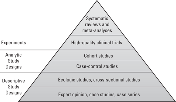
Each of the study designs discussed in the previous sections generates a particular level of evidence for causal inference. These levels of evidence may be arranged in a pyramid. As shown in Figure 7-2, the study designs with the strongest evidence for causal inference are at the top of the pyramid, and those with the weakest are at the bottom.
© John Wiley & Sons, Inc.
FIGURE 7-2: Levels of evidence in study designs.
Starting at the base: Expert opinion
At the base of the study design evidence pyramid shown Figure 7-2 is a descriptive study design: expert opinion. When the condition of dementia was first identified, few clinicians had seen patients with dementia. These clinicians served as experts who would write about the dementia patients they treated and share their experiences at medical conferences. This is what is meant by expert opinion, and while it is helpful when conditions are first identified, expert opinion is considered a very weak descriptive study design.
Making the case with case studies
Also at the base of Figure 7-2 are case studies and case series. To develop an understanding of dementia when it was first identified, clinicians treating patients needed to study them. They would write up case studies or case reports on individual patients describing their symptoms and providing the best descriptive evidence as possible. If the clinician was able to identify more than one patient, they could write about a series of patients, which is known as a case series. While case studies and case series are helpful for researchers when a condition is first identified, they are considered as providing very weak evidence to use for causal inference.
Making statements about the population
Ecologic studies (also called correlational studies) and cross-sectional studies appear in the next level up from expert opinion and case studies and case series. Though ecologic studies are still descriptive designs that provide weak evidence, they have the advantage of having potentially very large samples.
In ecologic studies, the experimental units are often entire populations (such of a region or country). For example, in a study presented in Chapter 16 of Epidemiology For Dummies by Amal K. Mitra (Wiley), the experimental unit is a country, and 15 countries were included in the analysis. The exposure being investigated is fat intake from diet (which was operationalized as average saturated fat intake as a percentage of energy in the diet). The outcome was deaths from coronary heart disease (CHD), operationalized as 50-year CHD deaths per 1,000 person-years (see Chapter 15 for more about rates in person-years). Figure 7-3 presents the results in the form of a scatter plot.

© John Wiley & Sons, Inc.
FIGURE 7-3: Ecologic study results.
As shown in Figure 7-3, the country’s average value of the outcome (rate of CHD deaths) is plotted on the y-axis because it’s the outcome. The exposure, average dietary fat intake for the country, is plotted on the x-axis. The 15 countries in the study are plotted according to their x-y coordinates. Notice that the United States is in the upper-right quadrant of the scatter plot because it has high rates of both the exposure and outcome. The strong, positive value of correlation coefficient r (which is 0.92) indicates that there is a strong positive bivariate association between the exposure and outcome, which is weak evidence for causality (flip to Chapter 15 for more on correlation).
 But the problem with ecologic studies is that the experimental unit is a whole population — not an individual. What if the individuals in the United States who ate low-fat diets were actually the ones to die of CHD? And what if the ones who ate high-fat diets were more likely to die of something else? Attributing the behavior of a group to an individual is called the ecologic fallacy, and can be a problem with interpreting results like the ones shown in Figure 7-3.
That is why we also have cross-sectional studies, where the experimental unit is an individual, not a population. A cross-sectional study takes measurements of individuals at one point in time — either through an in-person hands-on examination, or by survey (over the phone, Internet, or in person). The National Health and Nutrition Examination Survey (NHANES) is a cross-sectional surveillance effort done by the U.S. government on a sample of residents every year. NHANES makes many measurements relevant to human health in the United States, including dietary fat intake as well as status of many chronic diseases including CHD. If an analysis of cross-sectional data like NHANES found that there was a strong positive association between high dietary fat intake and a CHD diagnosis in the individuals participating, it would still be weak evidence for causation, but would be stronger than what was found in the ecologic study presented in Figure 7-3.
Going from case series to case-control
The reason that there are two types of analytic study designs — case-control studies and cohort studies — is that cohort study designs do not work for statistically rare conditions. We use the term statistically rare because if someone you love gets cancer, cancer does not seem very rare. Yet, if you enroll a cohort of thousands of individuals including your loved one (who is free of cancer) in a cohort study and measure this cohort yearly to see who is diagnosed with cancer, it would take many years to get enough outcomes to be able to develop the regression models (like the ones described in Chapters 16 through 23) that would be necessary for causal inference. So for statistically rare conditions like the various cancers, you use the case-control design.
You can use a fourfold, or 2x2, table to better understand how case-control studies are different from cohort studies. (Refer to Chapters 13 and 14 for more about 2x2 tables.) As shown in Figure 7-4, the 2x2 table cells are labeled relative to exposure status (the rows) and outcome or disease status (the columns). For the columns, D+ stands for having the disease (or outcome), and D– means not having the disease or outcome. Also, for the rows, E+ means having the exposure, and E– means not having the exposure. Cell a includes the counts of individuals in the study who were positive for both the exposure and outcome, and cell d includes the counts of individuals who were negative for both the exposure and outcome (a and d are concordant cells because the exposure and outcome statuses agree). In the discordant cells, where the exposure and outcome do not agree, is b, which represents the count of those positive for the exposure but negative for the outcome, and c, which represents the count of those negative for the exposure but positive for the outcome.

© John Wiley & Sons, Inc.
FIGURE 7-4: 2x2 table cells.
The 2x2 table shown in Figure 7-4 is generic — meaning it can be filled in with data from a cross-sectional study, a case-control study, a cohort study, or even a clinical trial (if you replace the E+ and E– entries with intervention group assignment). How the results are interpreted from the 2x2 table depend upon the underlying study design. In the case of a cross-sectional study, an odds ratio (OR) could be calculated to quantify the strength of association between the exposure and outcome (see Chapter 14). However, any results coming from a 2x2 table do not control for confounding, which is a bias introduced by a nuisance variable associated with the exposure and the outcome, but not on the causal pathway between the exposure and outcome (more on confounding in Chapter 20).
Imagine that you were examining the cross-sectional association between having the exposure of obesity (yes/no), and having the outcome of HTN (yes/no). Household income may be a confounding variable, because lower income levels are associated with barriers to access to high-quality nutrition that could prevent both obesity and HTN. However, in a bivariate analysis like is done in a 2x2 table, there is no ability to control for confounding. To do that, you need to use a regression model like the ones described in Chapters 15 through 23.
So how would you use a 2x2 table for a case-control study on a statistically rare condition like liver cancer? Suppose that patients thought to have liver cancer are referred to a cancer center to undergo biopsies. Those with biopsies that are positive for liver cancer are placed in a registry. Suppose that in 2023 there were 30 cases of liver cancer found at this center that were placed in the registry. This would be a case series. Imagine that you had a hypothesis — that high levels of alcohol intake may have caused the liver cancer. You could interview the cases to determine their exposure status, or level of alcohol intake before they were diagnosed with liver cancer. Imagine that 10 of the 30 reported high alcohol intake. You will see that as some evidence for your hypothesis.
But you could not do causal inference unless you had a comparable comparison group without liver cancer so that you could fill out your 2x2 table. Imagine that you went back to the cancer center and were able to contact and enroll 30 patients who had liver biopsies but were found not to have liver cancer to serve as controls. Suppose that you interviewed this group and discovered that only two of them reported high levels of alcohol intake. You could develop the 2x2 table like the one shown in Figure 7-5.

© John Wiley & Sons, Inc.
FIGURE 7-5: Example of a typical case-control study 2x2 table.
As shown in Figure 7-5, what is important is not the 2x2 table itself, but the order in which the counts are filled in. Notice that at the beginning of the study, you already knew the case total was 30, and you had determined that your control total would be 30 (although you are allowed to sample more controls if you want in a case-control study).
The correct measure of relative risk to present for a case-control study is the OR (as described in Chapter 14). It is important to acknowledge that when you present an OR from a case-control study, you interpret it as an exposure OR, not an outcome or disease OR. (It is also acceptable to present an OR in a cross-sectional study, but in that case, you are presenting an outcome or disease OR.)
In a case-control study, because the condition is rare, you are sampling on the outcome and calculating the likelihood that the cases compared to controls were exposed. This study design is seen as extremely biased, which is why cohort studies are preferred, and are at a higher level of evidence. However, case-control study designs are necessary for rare diseases.
Following a cohort over time
In the previous section, we pointed out that case-control studies are used for rare diseases. Therefore, case-control studies do not have large sample sizes, which is evident in Figure 7-5 where the total sample size is 60. In contrast, cohort studies are used for studying common conditions, such as HTN, so they include very large sample sizes — but they still use the same 2x2 table for interpretation. Figure 7-6 offers an example of what a 2x2 table for a cohort study might look like where the exposure is high alcohol intake and the outcome is HTN.

© John Wiley & Sons, Inc.
FIGURE 7-6: Example of a typical cohort study 2x2 table.
As shown in Figure 7-6, the total number of participants is large. This cohort of 600 participants could have been naturally sampled from the population, or they could be stratified by exposure, meaning that the study design could require a certain number of participants to be exposed and to be unexposed. Imagine that you insisted that 300 of your participants have high alcohol intake, and 300 have low alcohol intake. It may be harder to recruit for the study, but you would be sure to have enough exposed participants for your statistics to work out. In the case of Figure 7-6, 210 exposed and 390 unexposed participants were enrolled.
In cohort studies, all the participants are examined upon entering the study, and those with the outcome are not allowed to participate. Therefore, at the beginning of the study, all 600 of the participants did not have the outcome, which is HTN. A cohort study is essentially a series of cross-sectional studies on the same cohort called waves. The first wave is baseline, when the participants enter the study (all of whom do not have the outcome). Baseline values of important variables are measured (and criteria about baseline values may be used to set inclusion criteria, such as minimum age for the study). Subsequent waves of cross-sectional data collection take place at regular time intervals (such as every year or every two years). Changes in measured baseline values are tracked over time, and subgroups of the cohort are compared in terms of outcome status. Figure 7-6 shows the exposure status from baseline, and the outcome status from the first wave.
Because the exposure is measured in a cohort study before any participants get the outcome, it is considered the highest level of evidence among the observational study designs. It is far less biased than the case-control study design. Several measures of relative risk can be used to interpret a cohort study, including the OR, risk ratio, and incidence rate (see Chapter 14).
Advancing to the clinical trial stage
Higher up the pyramid of evidence shown in Figure 7-2 are experiments. Not all experiments are at such a high level of evidence — only high-quality clinical trials. These are experiments, not observational studies. This is where the researcher assigns the participants to engage in a particular behavior or intervention during the study. There are different types of clinical trials as described in Chapter 5; however, the highest-quality trials use both double-blinding and randomization. Double-blinding is where both the researcher and the participant do not know whether the participant was assigned to an active intervention (one being studied), or a control intervention. Randomization is where participants are randomly assigned to groups (so there is no bias in selecting participants for each group).
It is possible to use a 2x2 table to analyze the results of a high-quality clinical trial as long as the rows are replaced with the intervention groups. You can report the same measure of relative risk as for a cohort study; however, the difference is that the high-quality clinical trial would be seen as having much less bias than the cohort study — and stronger causal evidence.
Reaching the top: Systematic reviews and meta-analyses
Imagine a scenario where a new drug for HTN was developed, and several clinical trials were conducted to see whether this drug was better than the most popular current drug used for HTN. How would we be able to know whether, on balance, the new drug was actually better when we have so many different clinical trials on the same drug with different results?
We could ask a similar question about observational studies as well. Imagine that multiple case-control studies were conducted to determine whether having liver cancer was associated with the exposure of having high prediagnosis alcohol intake. What is the overall answer? Does high alcohol intake cause liver cancer or not? You could also imagine that multiple cohort studies could be conducted examining association between the exposure of high alcohol intake and developing the outcome of HTN. How would the results of these cohort studies be taken together to answer the question of whether high alcohol intake actually causes HTN?
The answer to this question are systematic reviews and meta-analyses. In a systematic review, researchers set up inclusion and exclusion criteria for reports of studies. Included in those criteria are requirements for a certain study design. For interventions, randomized clinical trials containing a control group (called randomized controlled trials, or RCTs) are usually required, but for other exposures, either case-control or cohort study designs are required. With respect to medications, RCTs are required as part of regulatory approval for distribution (see Chapter 5), so expect to see meta-analyses arising from results from clinical trials. In a systematic review, the studies included are compared and summarized in a table, but their numerical estimates coming from their results are not combined. The meta-analysis is the same as a systematic review except the numerical estimates coming from the results reported are combined statistically to produce an overall estimate based on the studies included. Systematic reviews and meta-analyses are described in more detail in Chapter 20.
If you are looking for the highest quality of evidence right now about a current treatment or exposure and outcome, read the most recent systematic reviews and meta-analyses on the topic. If there aren’t any, it may mean that the treatment, exposure, or outcome is new, and that there are not a lot of high quality observational or experimental studies published on the topic yet.